graphs_m12.html

> restart;

Comments. Remember, that in order to interact with worksheets, you have to reexecute all the commands. The commands in this worksheet and the other MTH 243 worksheets are entered in the classical 1-D Maple input that is common to all versions of Maple. You can use the 2-D input if you prefer. To convert from one to the other, right-click on the command line, choose Covert -> 2-D Math Input.

Reminder. In the classical 1-D Maple input, you have to end each command with a semicolon (or colon to suppress the output).

GRAPHS OF FUNCTIONS OF TWO VARIABLES

As you know, visual representation of functions of two variables is not an easy matter. The graph of a given function of two variables, say f(x,y), is a surface in the (x,y,z)-space. The graph is the set of all points (x,y,z) such that . In other words, the graph is the set of all points of the form (x,y,f(x,y)). Drawing such graphs "by hand" can be very difficult, if not impossible. Maple can be of great help in this respect. As you will see, Maple can plot spectacular graphs and rotate them at a touch of the mouse.

In our first example we are dealing with a function of two variables C=f(x,t). First, we shall analyze the behavior of the function using cross-sections f(a,t), f(x,b). Cross-sections, as you know, usually provide a lot of insight into the behavior of a function of two variables. Next, we shall have Maple plot the graph of the function.

Example 1. A drug is injected into muscle tissue. Typically, the concentration of the drug in the blood increases until it reaches its peak, and then begins to decrease as the body's metabolic processes remove the drug from the body. The concentration, C, in mg per 100 ml of blood, is a function of the amount of the drug injected, x, measured in 100's of mg, and the time, t, measured in hours since the injection was administered. That is

Suppose that for a certain drug a good mathematical model for the concentration following an injection is given by

for 1< x < 4 , t > 0.

That is, the formula is valid for initial injections between 100 and 400 mg, and for all times t.

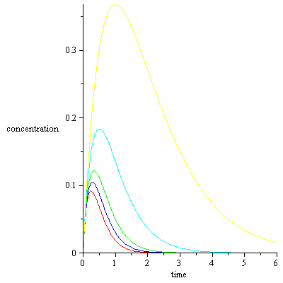
(a) Plot and interpret in practical terms a few cross-sections with the amount of initial injection fixed, e.g., f(1,t), f(1.5,t), f(2,t), f(3,t), f(4,t).

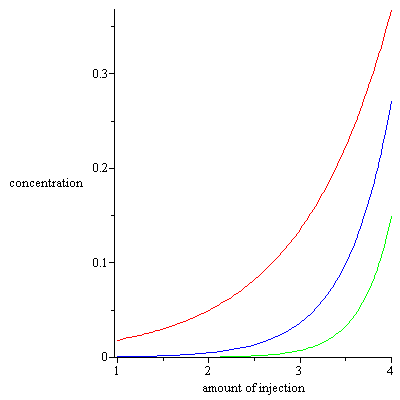
(b) Plot and interpret in practical terms a few cross-sections with time fixed, e.g., f(x,1), f(x,2), f(x,3).

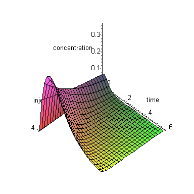
(c) Plot the graph of the function C = f(x,t) in the ( x,t,C)-space. Compare the graph with the cross-sections obtained above.

We begin by defining the function . The syntax is similar to the syntax in the case of one variable.

> f:=(x,t)->t*exp(-t*(5-x));

(1)

Next, we plot cross-sections required in (a). Observe that for each of the cross-sections, say f(1,t), the value x of the initial injection is fixed. Hence, the corresponding cross-section is a function of one variable only. Maple is perfectly aware of that. Indeed:

> f(1,t); f(1.5,t);

(2)

To plot the cross-sections, we use the plotting syntax that we learned last year. We have to guess the range for t. We are looking for a range after which the amount of the drug has decayed practically to 0 for all initial injections. Let's try t = 6 hours.

> plot([f(1,t),f(1.5,t),f(2,t),f(3,t),f(4,t)],t=0..6,color=[red,blue,green,cyan,yellow], labels=["time","concentration"]);

Plot_2d

Note how the peak concentration, and the time at which the peak concentration occurs vary as you vary the initial dose x. The peak concentration is, of course, higher for larger initial injections, and the larger initial injection, the longer it takes for the drug to dissipate. Within the range of this model, the time of peak concentration is never much past 1 hour.

Let's look at the cross-sections (b), where the time is fixed at, respectively, t = 1,2,3 hours after an injection and the amount of initial injection, x, varies. The proper range for x, from 1 to 4, is clear.

> plot([f(x,1),f(x,2),f(x,3)],x=1..4,color=[red,blue,green],labels=["amount of injection","concentration"]);

Plot_2d

Remember, the red graph shows concentration at time 1 for all possible initial injections x. The blue graph shows concentration at time 2 for all x, and so on. Not surprisingly, for any fixed moment in time the concentration is larger for larger amounts of the initial injection. The blue and green graphs, which show concentration at, respectively, 2 and 3 hours after an injection, are flatter than the red graph which shows concentration near its peak t =1.

We shall see now how all that information translates into properties of the graph of the function C = f(x,t) of two variables. The syntax for plotting functions of two variables is similar to the syntax in the case of one variable. The basic command is plot3d. There are many options and attributes that can be added to a 3d plot. We shall learn them as we go along.

We will show how to apply various options from Maple classical input. In Maple 12, you can play with the options by clicking on the plot and choosing various options fro the tool menu above. There are even more options available if you right-click on the plot and use the menu that appears.

> plot3d(f(x,t),x=1..4,t=0..6,labels=["injection","time","concentration"],axes=normal);

Plot

The beauty of Maple's 3d plots is that you can rotate them by simply moving the mouse, thereby changing the viewpoint from which you are looking at a surface. Left-click at any point on the above graph. Now, move the mouse holding down the left button. The graph will rotate allowing you to see the surface from any viewpoint you want. This is a great way to understand the shape of a surface.

As you click on the graph, a blue frame appears around it, as well as a menu on the toolbar. The menu allows you to change many attributes of the graph. Experiment with the menu on your own. In the worksheets, we shall use commands rather than menus to set the properties of plots.

Look carefully at the 3d graph above. Do you see the cross-sections with x fixed and with t fixed that we drew before as functions of one variable?

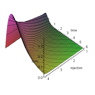
Since the axis can't be seen behind the plot, let's change the type of axes to "framed" by typing axes=framed on the command line. If a graph is a little choppy, you can improve its appearance by using the grid option. The grid corresponds to the number of points at which Maple evaluates a given function. If you have a very fast-changing function, it may be important to choose a finer grid. The syntax is grid=[ .. ,.. ].

> plot3d(f(x,t),x=1..4,t=0..6,labels=["injection","time","conc"],axes=framed,grid=[40,40]);

Plot

The plot seems clearer now. With framed or boxed types of axes, Maple will not display names for the vertical axis that are too long. Hence, we have abbreviated the name to "conc".

To learn more about various options for 3d graphs, and there are plenty of them, use Maple's on-line help by typing ?plot3d,option .

Example 2. A string is pegged along the x-axis with the endpoints at x=0 and x=1. You pluck the string in a certain way so it vibrates according to the formula:

v(x,t) = cos(t) sin(2*Pi* x),

where t is the time, in milliseconds, x the horizontal coordinate of a point on the string. v(x,t) denotes the vertical displacement of the point x at time t. (We are assuming that each point vibrates only in the vertical direction.)

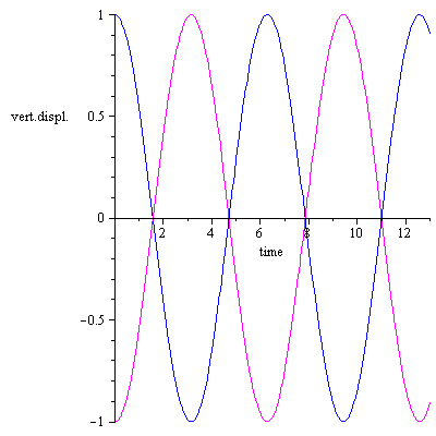
(a) Plot a few cross-sections with x fixed, say v(0.25,t), v(0.5,t), v(0.75,t). Explain their meaning in practical terms. Why one of the graphs doesn't seem to show at all?

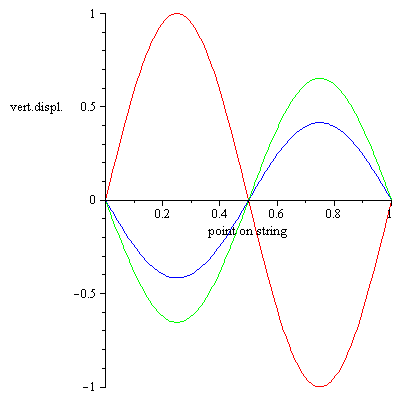
(b) Plot a few cross-sections with t fixed, say v(x,0), v(x,2), v(x,4). Explain their meaning in practical terms.

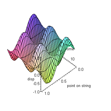
(c) Plot the 3d graph of the function v(x,t) for x between 0 and 1 and t between 0 and, say, 13. Rotate the graph to see clearly the cross-sections with x fixed and with t fixed.

We define the function v(x,t) in Maple:

> v:=(x,t)->cos(t)*sin(2*Pi*x);

(3)

Let's plot the cross-sections with x fixed.

> plot([v(0.25,t),v(0.5,t),v(.75,t)],t=0..13,color=[blue,green,magenta],labels=["time","vert.displ."]);

Plot_2d

The blue graph shows the motion of the point x=0.25 on the string during the first 13 milliseconds. We see the point going down from the initial displacement of 1 and then up again, then down, and so on. The magenta graph shows the vertical motion of the point x=0.75 on the string during the first 13 milliseconds. Why is the graph of the crosssection v(0.5,t) not showing? Look at the formula carefully. For x=0.5, v(0.5,t)=0 for all t. In other words, the middle point of the string does not vibrate at all. At this point we have a so-called node. The graph of v(0.5,t) doesn't show as it coincides with the t-axis. As we see, cross-sections with x fixed show the vertical vibration of each given point on the string.

Let's plot a few cross-sections with t fixed.

> plot([v(x,0),v(x,2),v(x,4)],x=0..1,color=[red,blue,green],labels=["point on string","vert.displ."]);

Plot_2d

The red graph shows the veritcal position of each point on the string at the initial moment t=0. In other words, it shows the shape of the string at t=0. The blue graph shows the shape of the tring at time t=2, and so on. As we see, cross-sections with t fixed show the shape of the string at each given moment.

Next, let's have Maple plot a 3d graph of v(x,t).

> plot3d(v(x,t),x=0..1,t=0..13,axes=framed,labels=["point on string","time","disp"]);

Plot

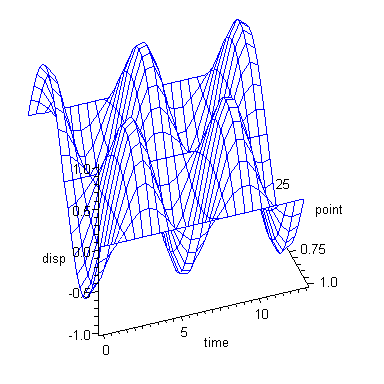
Rotate the above graph. You obtain some beautiful views clearly showing the cross-sections with t fixed, which give the shape of the string at each moment, as well as cross-sections with x fixed illustrating vibrations of each given point. As you rotate the graph, the two numbers at the upper left corner of your screen next to the two Greek letters change. The numbers represent vertical and horizontal angles describing your viewpoint. We can lock in any given view in the command line using the orientation option and the two numbers corresponding to the view. (Otherwise, reexecuting the command will erase the results of rotation.) For example, when rotating the above graph we notice that two really good views correspond to orientation=[-75,100] and orientation=[-20,50]. We display the latter view below. In order to practice different options for 3d graphs, we display it in a different style than the graph above. The style option is a very important option for 3d graphs. All the graphs above were shown in the style=patch style. It is the default option in Maple so we didn't have to specify it. The graph below is displayed in style=hidden, which shows the graph as a wireframe in such a way that parts of the surface that are obscured from view by the surface remain hidden. Another option that we use below is the color option.

> plot3d(v(x,t),x=0..1,t=0..13,axes=framed,orientation=[-20,50],style=hidden,color=blue,labels=["point","time","disp"]);

Plot

Remark. As you know, not all surfaces in the (x,y,z)-space are graphs of functions of two variables. A similar vertical line test applies as in the case of functions of one variable. Maple can plot surfaces defined by (x,y,z)-equations using the implicitplot3d command contained in the with(plots) package.

Homework Problems

Note. Homework problems call for explanations. Make sure that your explanations are clear. Use complete sentences. Type all explanations and comments in Maple in your homework worksheet.

Note: exp(-0.12 t) stands for . When entering the constant 'Pi' remember, it is Pi and not pi.

Problem 1. A laterally insulated copper bar 80 cm long is located along the x axis with one end at x=0 and the other x=80. The ends of the bar are kept at constant temperature of 0 degrees Celsius. Assume that the temperature at any point x on the bar at time t, measured in minutes, is given by

u(x,t) = 100 sin( Pi * x / 80 ) exp( -0.12 t).

(a) Plot a few cross-sections with t fixed in one coordinate system, e.g., u(x,0), u(x,5), u(x,10), u(x,20). Explain their meaning in practical terms. In particular, what does u(x,0) tell you?

(b) Plot a few cross-sections with x fixed in one coordinate system, e.g., u(10,t), u(30,t), u(60,t), for t between 0 and 30. Explain their meaning in practical terms.

(d) By looking at the graph in (c), can you see at what point of the bar the temperature is always the highest? Can you explain this in physical terms? What happens to the temperature of the bar in the long run?

Problem 2. Consider the function

h(x,y) = cos( (x^2 + y^2 )^(0.5) ).

(a) Draw the graph of the function. Choose a range for x and y not too large, so that the shape of the function near x = 0, y=0 is clearly visible and the graph is not too choppy, but large enough so that the oscillatory behavior of the function is evident. What symmetries does the graph have?

(b) Rotate the graph of h(x,y) and lock in one interesting view with the orientation option.

Updated to Maple 12 by B. Kaskosz, January 2009.