SOLVING DIFFERENTIAL EQUATIONS USING MAPLE 

then you will learn how to plot the solutions. 

Let us first call the Differential Equations package: 

>	with(DEtools):

 

>

 

The derivative of an expression y(t) with respect to "t"  is denoted in Maple by diff(y(t), t). 

To enter the differential equation ty'+2y=sin(t)/t  into Maple  we type: 

>	e1:=t*diff(y(t),t)+2*y(t)=sin(t)/t;

 

(1)

 

>

 

Note that we refer to y consistently as y(t) in communicating with Maple. 

The second derivative of y(t)  with respect to  t is denoted in Maple as  diff(y(t), t,t)  

Let us enter in Maple the differential equation  2y''+3y'+t=t^2+3sin(t) 

>	e2:=2*diff(y(t), t,t)+3*diff(y(t), t)+t=t^2+3*sin(t);

 

(2)

 

>

 

It is time now to solve the differential equation ty'+2y=sin(t)/t  analytically. We do this by means of the command 

dsolve: 

>	dsolve(e1, y(t));

 

(3)

 

>

 

We will ask Maple now to find the particular solution of  2y''+3y'+t=t^2+3sin(t)   satisfying the initial conditions 

y(Pi)=0 and y'(Pi)=1 

>	dsolve({e2, y(Pi)=0, D(y)(Pi)=1}, y(t));

 

(4)

 

>	e2s:=rhs(%);

 

(5)

 

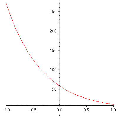
Note that in this case D(y) stands for y'  so,  D(y)(Pi)=1  stands for y'(Pi)=1. Let us now plot the solution that 

Maple has provided. 

>	plot(e2s, t=-1..1);

 

>

 

Solving differential equations numerically 

Exact analytic solutions to differential equations can sometimes not be found. Maple does not always succeed when instructed 

to find the solution using dsolve. For example let us try to find an analytic solution with Maple to the differential equation  

y''+xy'+y=0. 

>	e3:=diff(y(x), x, x)+diff(y(x), x)+ x^5*y(x)=0;

 

(6)

 

>	dsolve(e3, y(x));

 

(7)

 

>

 

As we can see, Maple cannot solve this equation and responds by recopying the problem. Most differential equations do not 

have explicit solutions in terms of known functions. 

In order to solve differential equations numerically, we need to have numerical initial conditions instead of symbolic 

constants. Let us tell Maple to solve the initial-value problem numerically  

>	e3s:=dsolve({e3, y(0)=3, D(y)(0)=-2}, y(x), numeric);

 

(8)

 

>

 

Maple returns a procedure  as its answer. To get values from that procedure we enter 

>

e3s(.5);

 

(9)

 

>

 

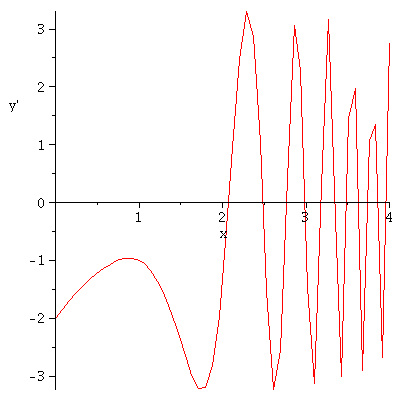
To plot y' versus x,  type 

>	with(plots):

 

>	odeplot(e3s,[x,diff(y(x),x)], 0..4);

 

>

 

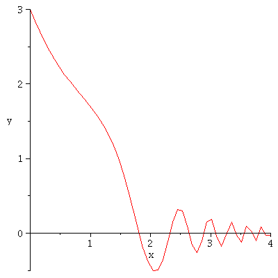
To plot the solution  y versus x, type 

>	odeplot(e3s,[x,y(x)], 0..4);

 

>

 

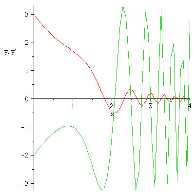
To plot both y and y' versus x, type 

>	odeplot(e3s,[[x,y(x)],[x,diff(y(x),x)]], 0..4);

 

>

 

HOMEWORK 

For each one of the problems below, use maple to solve the ODE. 

a) Find the general solution. If you can not find a nice analytic solution use the numerical approach that Maple 

provides and proceed as in the example previously discussed, extracting the answer for certain value of the variable, 

and then plotting y(t) versus t, y'(t) versus t and y(t) and y'(t) together versus t. 

b) Find the particular solution. 

c)Evaluate the particular solution at an appropriate value of  t. 

d)Plot the particular solution in an appropriate interval, so you get a good idea how the solution looks like. 

I) 

>

 

II) 

>

 

III) 

>

 

IV) 

>