>

restart;

 

>

 

Maple Syntax for Vectors and Gradients. Vectors are entered in Maple using the command vector . For example, to define the vector v=2 i +3 j -4 k in three-dimensional space, use the syntax  

>	v1:=vector([2,3,-4]);

 

(1)

 

Most commands to manipulate vectors are contained in the linalg  package ("linalg" for "linear algebra"). Let's load the linalg  package. If you are curious about its content, replace the colon by a semicolon on the line below before re-executing it. 

>	with(linalg):

 

>	norm(v1,2);

 

(2)

 

The "2" within the norm command stands for the root of order two in our definition of the magnitude. 

>	v2:=vector([1/2,3,-1]);

 

(3)

 

>	dotprod(v1,v2);

 

(4)

 

>	crossprod(v1,v2);

 

 

To add properly defined vectors , or to multiply them by scalars use the command evalm . 

 

(5)

>	evalm(3*v1-(1/2)*v2);

 

(6)

 

The useful command normalize returns a unit vector with the same direction as a given vector. In other words, divides a nonzero vector by its magnitude. For example:  

>	normalize(v1);

 

(7)

 

Another handy command is angle . The command calculates the angle between two vectors.  

>	angle(v1,v2); evalf(%);

 

 

	(8)

 

The value of the angle is returned in radians.The very important command grad that calculates the gradient of a given function of two or more variables is also contained in the linalg package. Remember that: 

If F is a function of two variables x and y, the gradient of F is the vector function whose first component is the partial derivative of F with respect to x and whose second component is the partial derivative of F with respect to y. 

>	grad(F(x,y), vector([x,y]));

 

(9)

 

Notice that the gradient vector of a function of two variables is itself a function of two variables. In fact, it's a function which takes two variables, x  and y , as input, and which outputs a vector. 

>	f:=(x,y)->x^4+y^4;

 

(10)

 

>	grad(x^4+y^4,[x,y]);

 

(11)

 

>	h:=(x,y,z)->exp(2*x)*sin(z*x*y^2);

 

(12)

 

>	gradh:=grad(h(x,y,z),[x,y,z]);

 

(13)

 

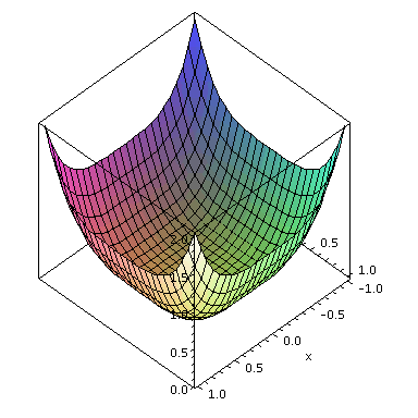
Let us plot our function f(x,y) 

>	plot3d(f(x,y), x=-1..1, y=-1..1, axes=BOX, scaling=constrained);

 

>	with(plots):

 

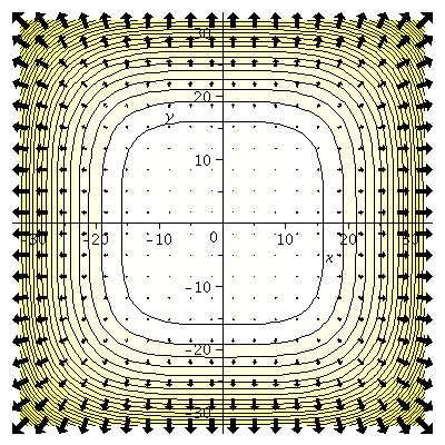
>	fcount:=contourplot(f(x,y), x=-32..32, y=-32..32, contours=30,filled=true,coloring=[white,yellow],scaling=constrained):

 

>	ffiledp:=fieldplot([4*x^3,4*y^3], x=-32..32, y=-32..32, color=BLACK, arrows=THICK):

 

>	display({fcount, ffiledp});

 

>

 

The gradient vector points in direction of greatest increase of "f" , which is away from the origin. As x  and y  increase, the gradient vector increases in length. The contour lines show paths in the plane along which the function is constant, so the direction of greatest increase of a function should be directly away from the contour lines. The length of the gradient vector indicates the steepness of the graph of "f", which increases as (x,y) moves away from the origin.  

For any unit vector u=[u1, u2] , the directional derivative of "f" at (a,b) in the direction u ,  f_u(a, b) , represents the rate of change of f in the direction u , and is given as the dot product of the vector u  with the gradient gradf(a,b), that is:

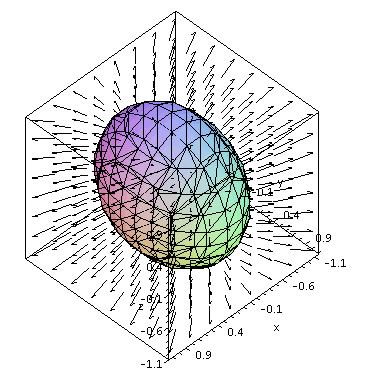
Example 2. Plot a level surface and the field of gradients for the function  

>	g:=(x,y,z)->2*x^2+y^2+z^2;

 

(14)

 

>	gradg:=grad(g(x,y,z),[x,y,z]);

 

(15)

 

>	gfieldp:=fieldplot3d(gradg,x=-1..1,y=-1..1,z=-1..1,scaling=constrained,axes=boxed,color=black):

 

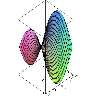
>	gplot:=implicitplot3d(g(x,y,z)=1,x=-1..1,y=-1..1,z=-1..1,axes=framed,scaling=constrained):

 

>	display([gfieldp,gplot]);

 

>

 

Homework Problems 

>

 

(16)

 

Display both its contour diagram and its field of gradients on the same plot. Comment on the direction in which you should move from a point (x,y) to obtain the maximum and minimum rates of change of f.  

Problem 2. 

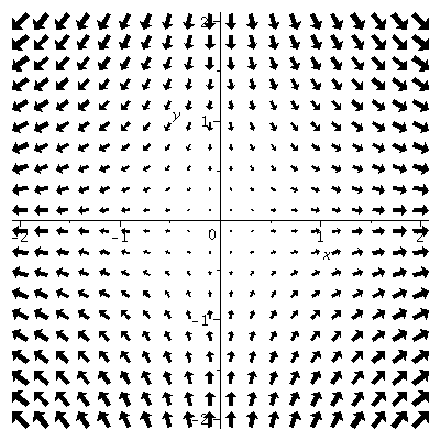
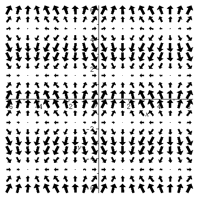
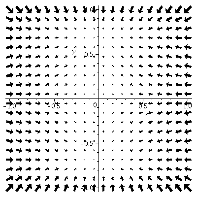
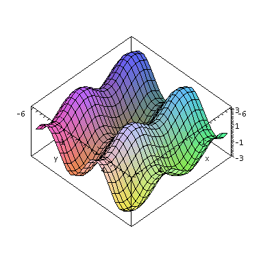
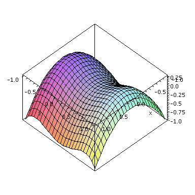
Match each of the sets of gradient vectors plotted below with the graph of a function 

                                                         (I) 

                                                        (II) 

>

 

                                                       (A) 

>	plot3d(sin(x)+2*sin(y), x=-6..6, y=-6..6, axes=boxed,scaling=constrained);

 

>

 

>	plot3d(y^2-y^4-x^2, x=-1..1, y=-1..1, axes=boxed, scaling=constrained);

 

>

 

>	plot3d((x^2-y^2), x=-2..2, y=-2..2, axes=boxed, scaling=constrained);